Building a BI pipeline in minutes

Learn how to transform data in AWS from DynamoDB and visualize it with QuickSight. Read this complete walk-through of setting up your first BI pipeline, with sample data provided. As you will notice, there’s no coding required to put up the BI pipeline itself. But of course, if you need more complex data transformation, you can customize the AWS Glue transformation script with Python or Scala.

The need

DynamoDB is the most popular NoSQL key-value pair database (according to DB-Engines Ranking), and indeed a very widely used database among serverless solutions developers in AWS universum. While DynamoDB can support usage peaks of even 20 million requests per second, it can sometimes be frustrating that there are no sophisticated ways of making simple queries based on non-key attributes to the data from AWS Console. And there are practically no ready capabilities to visualize the data and relations easily.

AWS launched in 2020 a service called PartiQL to make SQL kind of queries to DynamoDB, but the capabilities are still on “tech preview” level. There’s no way, for example, to make cross-table joins, the result sets also contain empty results, and DynamoDB scan restrictions bind the queries.

So, there’s plenty of room for a solution to enable making diverse SQL queries for DynamoDB data and visualize the data for business analytics and decision-making needs.

The cure

The solution is to build a BI pipeline to drive the data from DynamoDB to a business analytics platform. Eventually, you might consider moving the data to some enterprise-wide BI solution, let it be, for example, AWS Redshift for data warehousing and PowerBI for professional data visualization.

But as the first step for immediate needs and smaller organizations, you can build your first BI pipeline from end-to-end in less than one hour. The cure consists of the following AWS managed and easy-to-use ingredients:

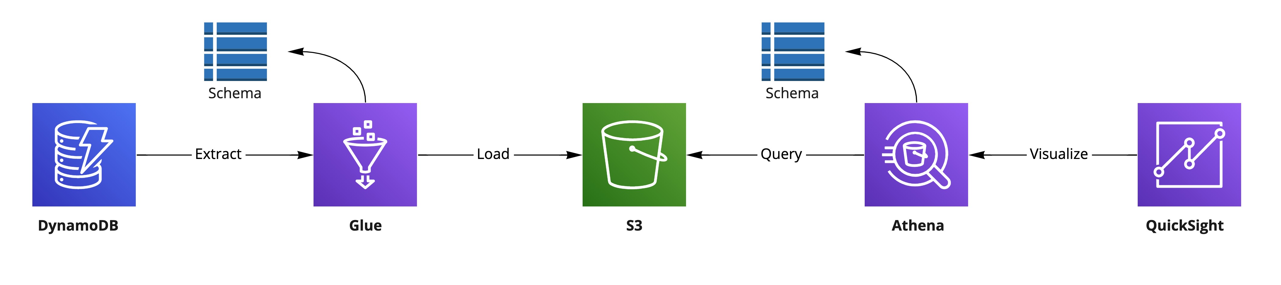
• AWS DynamoDB as the data source
• AWS S3 as the place to export data from DynamoDB
• AWS Glue for transforming the data from DynamoDB to S3
• AWS Glue Studio to build and execute the needed data pipeline with Glue
• AWS Athena to provide a diverse SQL interface for data in S3
• AWS QuickSight to visualize data available through Athena

The following figure illustrates the BI pipeline we are going to set up:

The steps

Here are the steps to get your DynamoDB data alive in QuickSight. The following steps contain instructions also for setting up a new DynamoDB table with some test data, in case you would like first to practice the process with the same data set as used in this example. If you already have a ready DynamoDB dataset to practice with, you can skip the first two steps and adjust the rest instructions with your use case.

1. Pre-step: Create a DynamoDB table

If you would like to follow these steps precisely, you should start by creating a new DynamoDB table on your AWS account. After creating the table, we need to import some test data to the table, and that operation is most effortlessly managed with the AWS CLI (command line interface), so let’s create the DynamoDB table also from the CLI.

You could set up the AWS CLI tools to run AWS commands directly from your laptop or use the AWS CloudShell available in AWS Console. I found it most accessible to open the CloudShell, wait for a few seconds for a virtual machine to set up for you, and run commands with no extra hassle.

When ready, run the following command (in one line) to create a DynamoDB table named Weather-demo, having Timestamp as the primary key for the table.

aws dynamodb create-table
--table-name Weather-demo
--attribute-definitions AttributeName=Timestamp,AttributeType=S
--key-schema AttributeName=Timestamp,KeyType=HASH
--provisioned-throughput ReadCapacityUnits=5,WriteCapacityUnits=5
--tags Key=Owner,Value=NordHero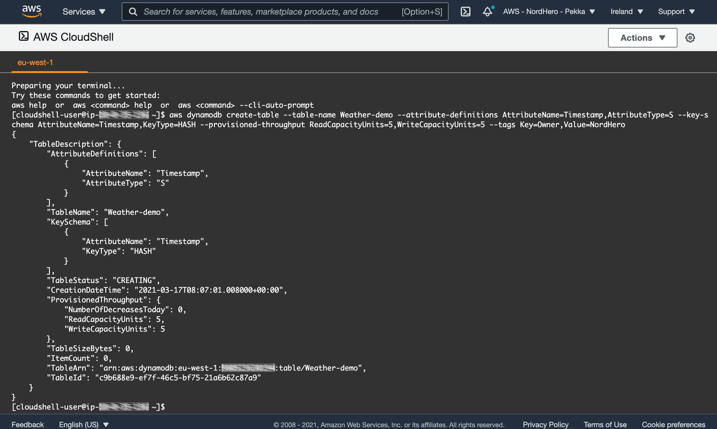

There you go, now we have a new table set up!

2. Pre-step: Insert demo data to the table

For the demo, I downloaded some open weather data from FMI (Finnish Meteorological Institute) and converted the data from Excel format to JSON to be easily uploadable to DynamoDB. This demo’s data set is weather observations for 2020 from one weather station located in Helsinki, Finland - one set of data per day, including temperatures and rain/snow amounts.

AWS CLI batch-write operation allows a max of 25 items inserted in one batch. Therefore, I needed to split the JSON into 16 files to have less than 25 items per file. You can download the pre-prepared data in a ZIP package from here.

If you are using AWS CloudShell, you can upload the ZIP package to the shell from Actions/Upload file. The uploaded file appears in your home directory. After getting the ZIP package in your CLI shell, unzip it to get the JSON files ready:

unzip weather-demo.zip

Each JSON struct has the target DynamoDB table (change the name from “Weather-demo” in each file if you have another table name) and at a maximum of 25 PutRequests per file, each containing one Item.

 1
 2
 3
 4
 5
 6
 7
 8
 9
10
11
12
13
14
15
16
17
18
19
20
21
22
23
24
25
26
27
28
29
30
31
32
33
34
35
36
37
38

{
"Weather-demo": [
{
"PutRequest": {
"Item": {
"Timestamp": {
"S": "2020-01-01T00:00:00Z"
},
"Rain (mm)": {
"N": "0"
},
"Snow depth (cm)": {
"N": "-1"
},
"Air temperature (degC)": {
"N": "1.5"
},
"Ground temperature min (degC)": {
"N": "-5.7"
},
"High temperature (degC)": {
"N": "3.4"
},
"Low temperature (degC)": {
"N": "-2.6"
}
}
 }
},
{
"PutRequest": {
"Item": {
// more data
}
}
}
]
}

Now you are ready to write the items to your DynamoDB table. Upload the first batch with the following command:

aws dynamodb batch-write-item --request-items file://1.json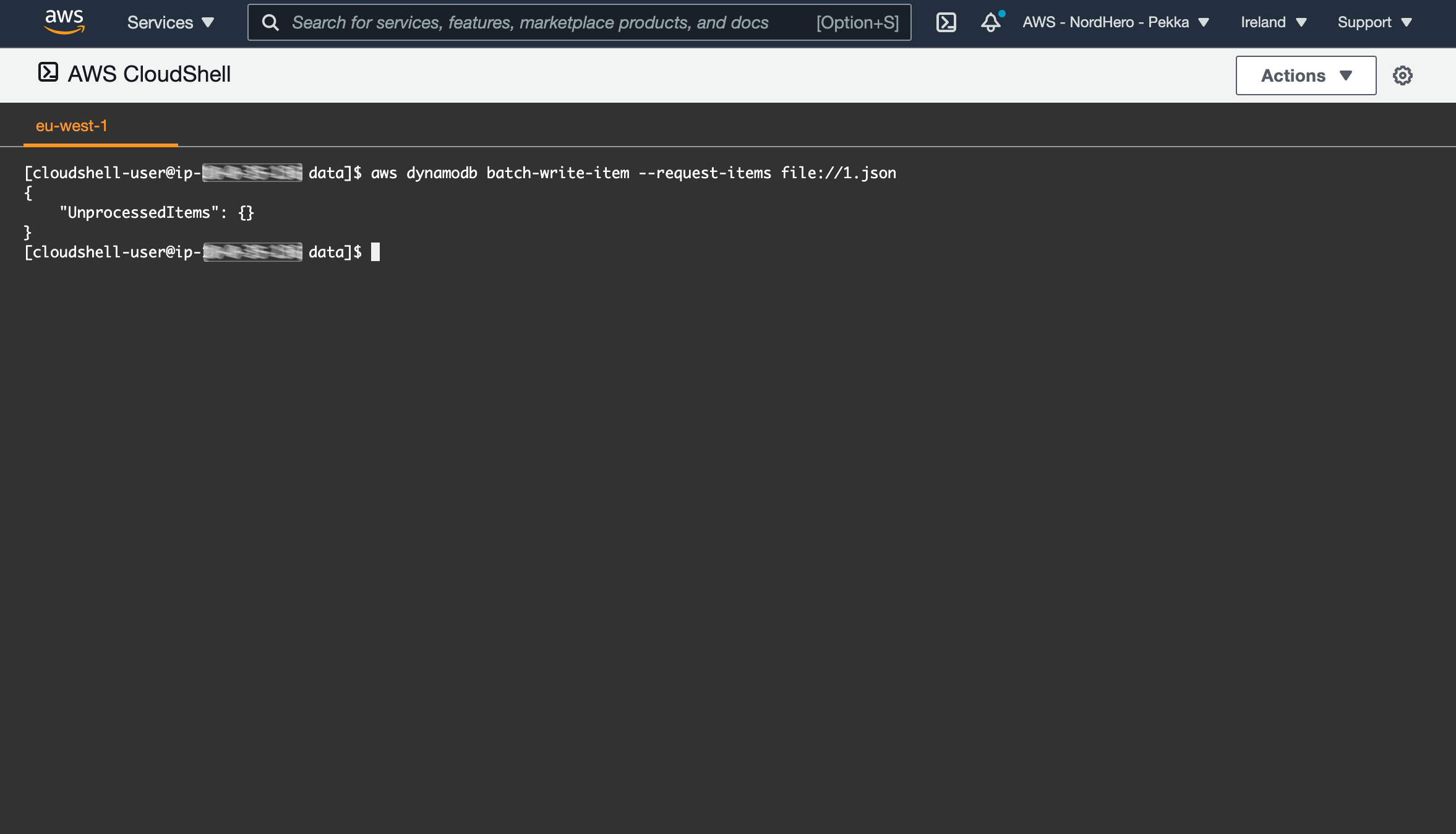

Repeat the same command for all 16 files. After running the commands, you can open the DynamoDB table in the AWS Console to see the items.

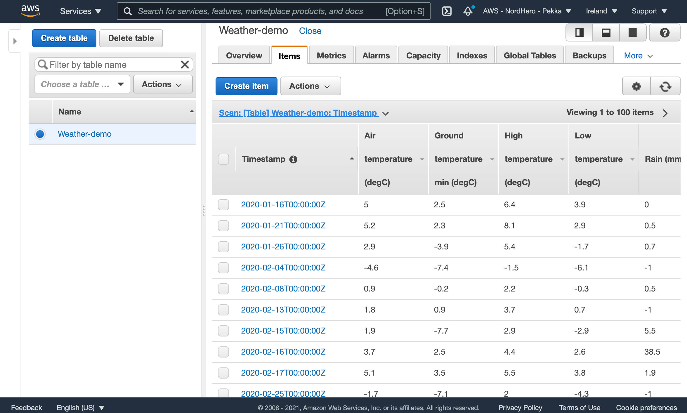
Now, we are ready to start building the BI pipeline!

3. Get the DynamoDB table schema with AWS Glue crawler

AWS Glue is a managed ETL solution (extract, transform, and load) to process data from various sources, combine, transform and normalize the data, and export the transformed data to be utilized in other systems. AWS Glue is a heavy-weight tool that manages parallel data processing utilities running on Apache Spark cluster, with data processing scripts written in Python or Scala. The needed processing capability is automatically set up and down by AWS Glue when Glue runs the jobs.

Before actually processing the data, AWS Glue needs to find out the schema for the data. Therefore, we need to set up a crawler in AWS Glue to snoop the data in our DynamoDB table and save the required meta information.

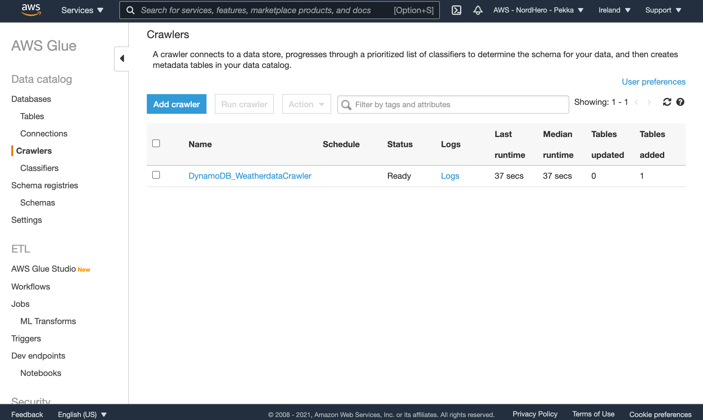
So open up AWS Glue in AWS Console and click Crawlers from the left-hand navigation menu. Then click Add crawler button and create a new crawler with the following information (if no information is given, you can leave those fields empty/default):

Crawler name: DynamoDB_WeatherdataCrawler
Crawler source type: Data stores
Choose a data store: DynamoDB
Table name: Weather-demo
Create an IAM role: AWSGlueServiceRole-WeatherDataRole
Frequency: Run on demand
Crawler’s output: Add database
Database name: weatherdb

Click Finish to create the crawler. Now you are ready to run the crawler by selecting the crawler and clicking Run crawler. The crawling might take 1-2 minutes, and after crawling, you should see that crawler found the source and created a metadata table in AWS Glue to represent the DynamoDB table schema.

You can now see a new database in AWS Glue’s Databases list and a new table in the Tables list. Open the weather_demo table from the Tables list and scroll down to see the meta-information captured from our DynamoDB table.

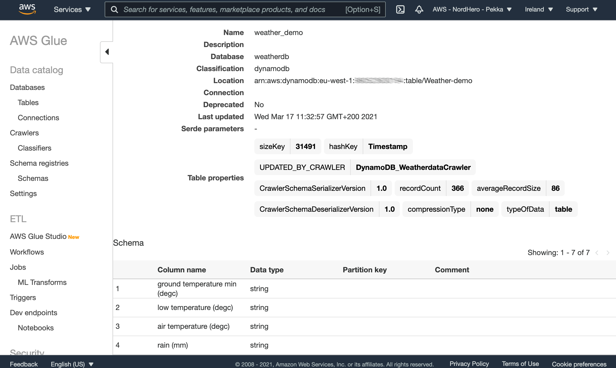
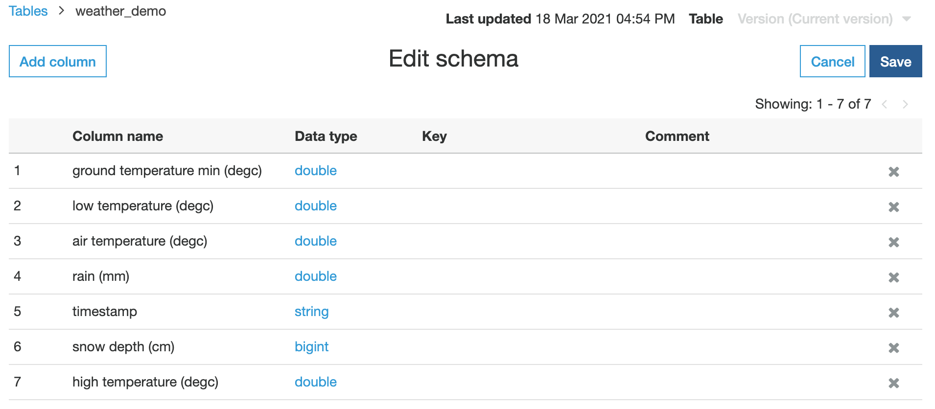
As you can see, there are altogether 366 records in our table (yep, 2020 had a leap day). You can also see that the crawler didn’t do a perfect job with column data types, as the crawler recognizes almost all numeric fields as string fields. So click Edit schema and change the data types from string to double for all numeric data types.

4. Prepare a S3 bucket for data loading

Next, we need to create a new S3 bucket to store the data transferred from DynamoDB. So open S3 from AWS Console, and create a new bucket with a unique name (S3 bucket names need to be globally unique). In my demo, I created a bucket with the name aws-glue-yourbucketnamehere.

Tip: Start the bucket name with “aws-glue-” because the IAM Role you created in the previous step has pre-set access rights (get, put, delete) set for buckets named with aws-glue-*. In case you named the bucket differently, you also need to update the mentioned IAM Role to have access to your bucket.

5. Get the data moving with AWS Glue Studio

Let’s start creating the Glue job that transfers the data from DynamoDB to S3. So open the AWS Glue again in AWS Console, and open AWS Glue Studio from the left-side navigation.

Click Create and manage jobs, select S3 for both Source and Target and click Create button.

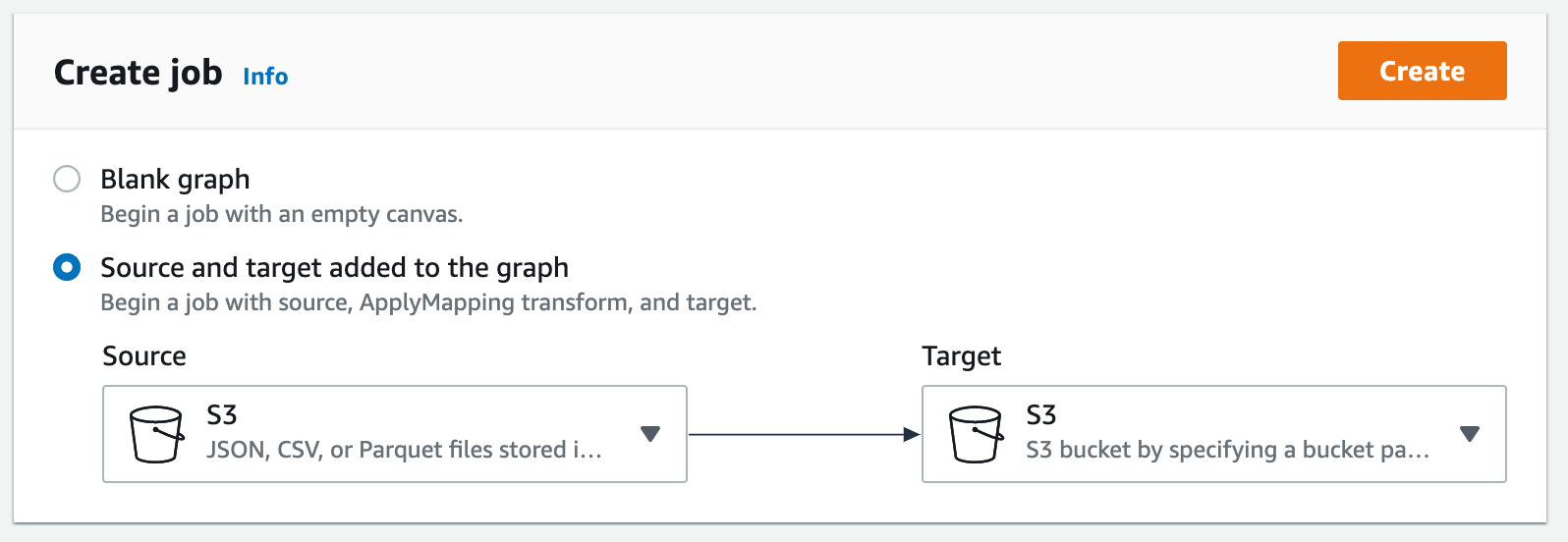
Now you will have a visual presentation of the data transformation job with Data source, Transform, and Data targets. Click on Data source and fill the following information into the form:

S3 source type: Data Catalog table
Database: weatherdb
Table: weather_demo

Next, click on Data target and fill in the following information:

Format: Parquet
Compression type: None
S3 Target Location: s3://aws-glue-yourbucketnamehere/

Now we have set the source and the target. Next, click on Transform and change Target key values to have easier column names to be used later on. Let’s also make one data type transform - change the Data type for timestamp field as timestamp:

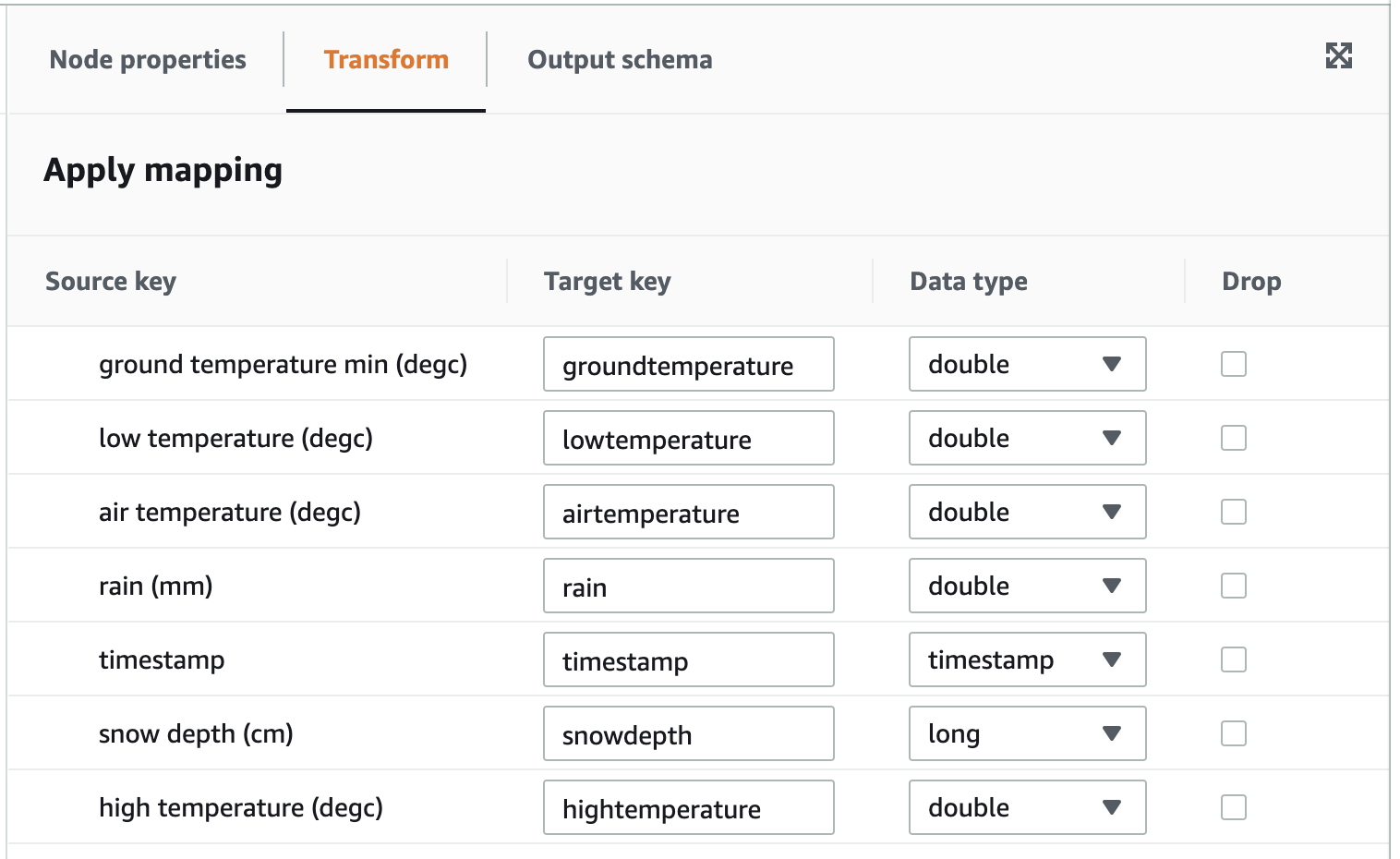
So we will keep all data fields in the transformation from the source database; we will change all data field names and do data type transformation for timestamp data.

As the last step, click on Job details tab and fill/change the following information:

Name: WeatherJob
IAM Role: AWSGlueServiceRole-WeatherDataRole
Number of workers: 2

The number of workers means that AWS Glue will spin up two virtual machines (workers) and give the workers a chunk of source data for parallel processing. The more you have workers; the less time is required to process.

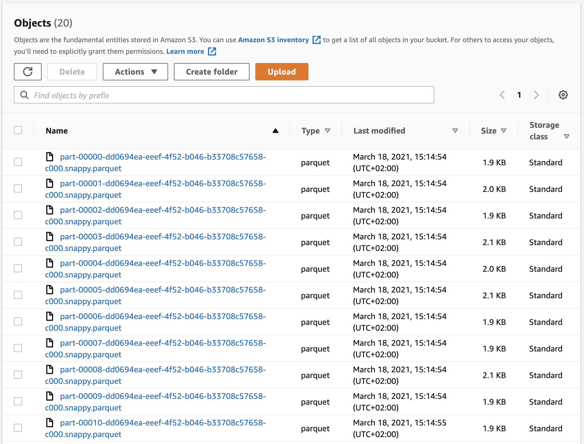
Now we are ready to rock! Click Save and Run. You can click the Run Details to follow the status of the data transformation process. When you get a green Succeeded status, you can browse to your S3 bucket and see that there’s a bunch of parquet files added.

Give yourself a little treat; you have successfully built a data pipeline from DynamoDB to S3! Next, we will prepare the data for visualization.

6. Get the schema for parquet data

Before setting up Athena to query the parquet data, we need to detect the schema for the data saved in S3. So get back to AWS Glue and create a new Crawler with the following info:

Crawler name: WeatherParquetCrawler
Crawler source type: Data stores
Choose a data store: S3
Include path: s3://aws-glue-yourbucketnamehere
Choose an existing IAM role: AWSGlueServiceRole-WeatherDataRole

Configure the crawler’s output/Database: weatherdb
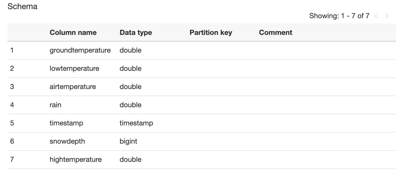
Grouping.../Create a single schema...: Checked

You can leave all other selections as-is. Click Save. Select the just created crawler and click Run crawler. After a while, you have a new Table in the Glue Database, named after your S3 bucket name and containing the schema information on the data in S3. You can check that the schema has all your data columns and that the data types are correct:

7. Make data available for SQL queries with Athena

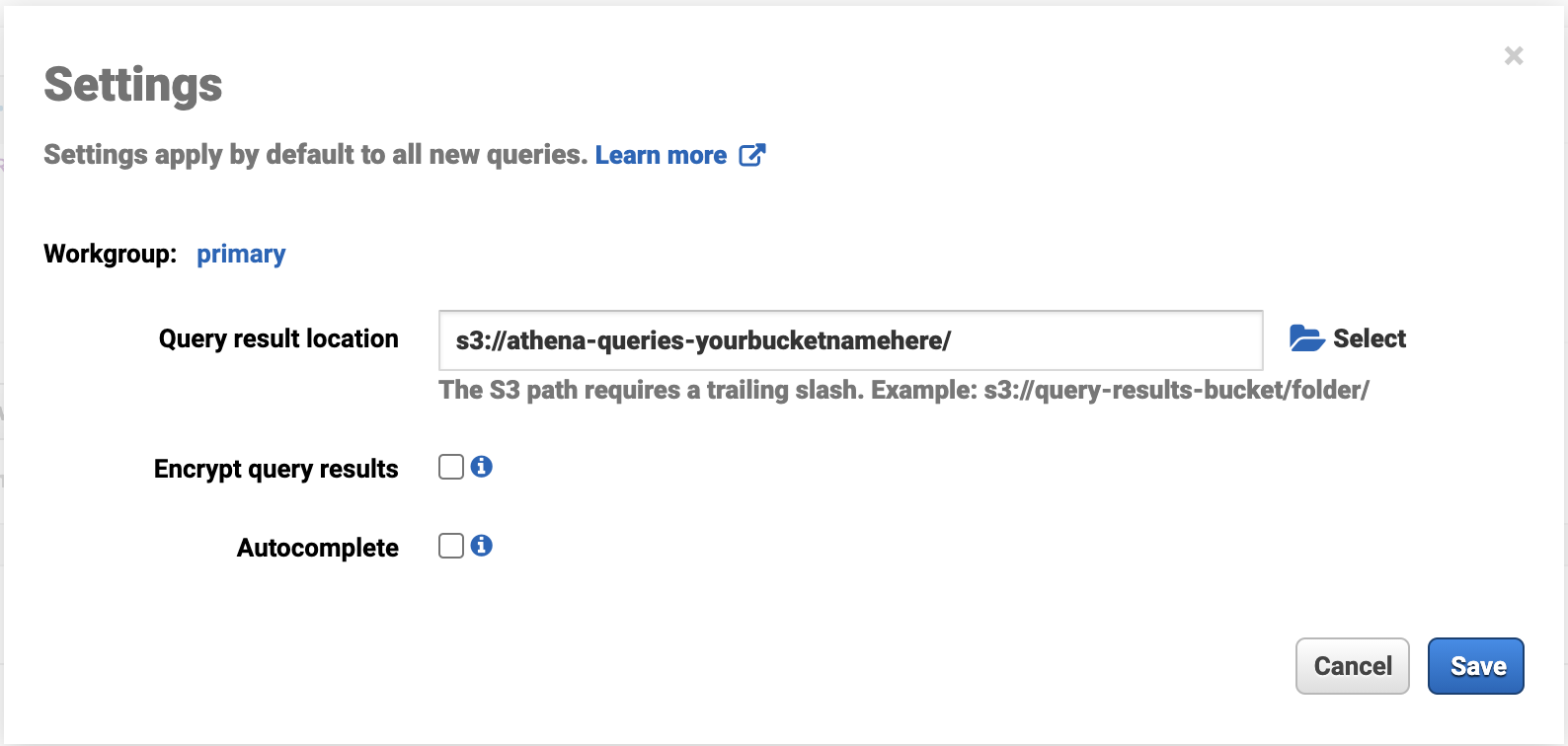
Before entering Athena, we need to create just one more S3 bucket. That bucket is going to be used by Athena for saving your queries and query results. So, please create a new S3 bucket and give it a name that indicates that it’s for Athena, so something like this, but unique: athena-queries-yourbucketnamehere.

After creating the bucket, you can open Athena in AWS Console. First, you need to give Athena the place to save queries, so open Settings and select your just created S3 bucket:

Now you can make your first query to the weather data. Select from the left-hand menu:

Data source: AwsDataCatalog
Database: weatherdb
Tables: aws_glue_yourbucketnamehere

Click on the three points next to the table name, and select Preview table. Athena automatically creates an SQL query to select ten rows from the table and shows the results below the query.

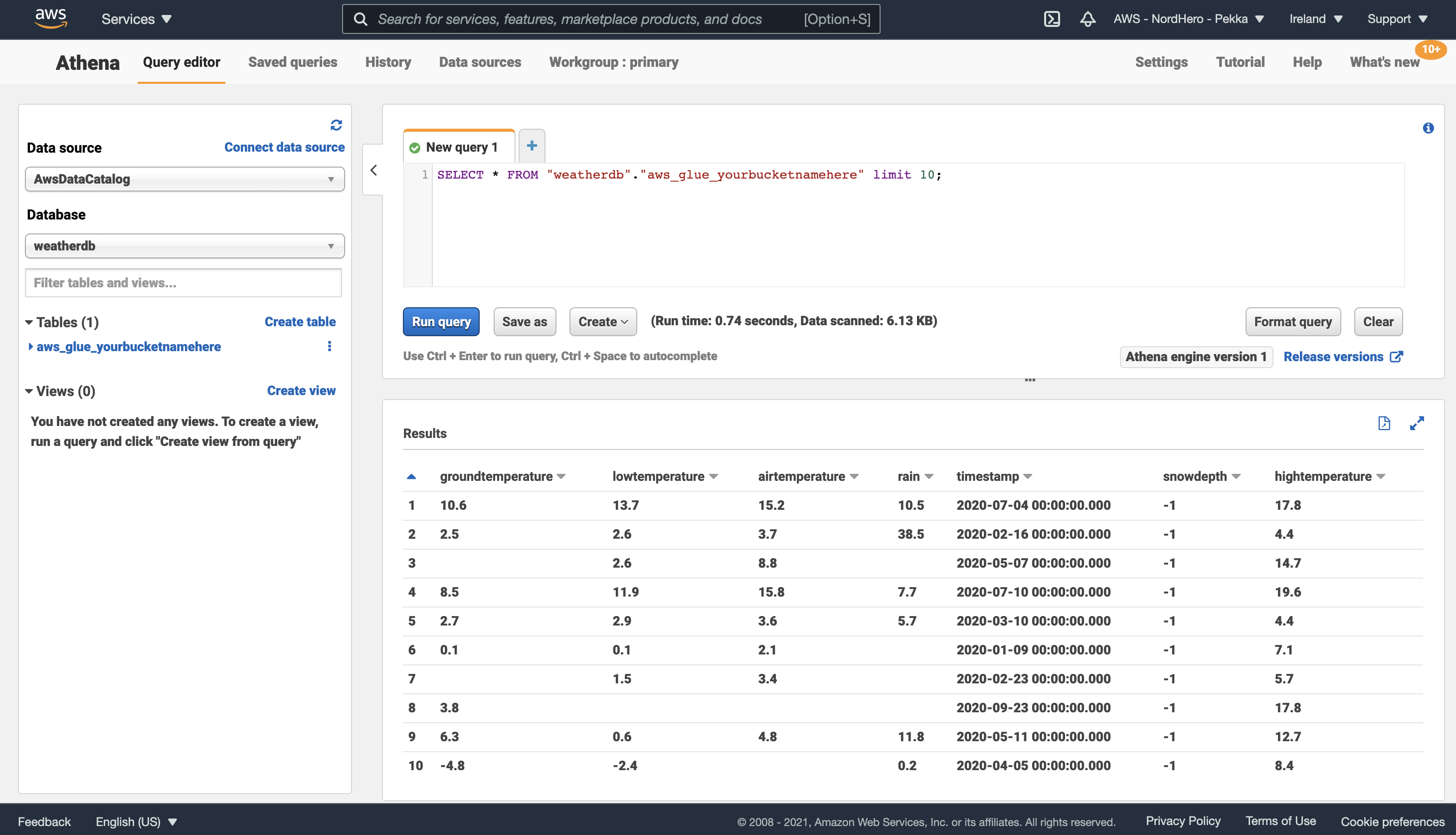
You can freely modify the SQL query and test the data querying capabilities. If you had several tables (even coming from different sources), you could easily join data from those tables with plain simple SQL.

8. Set up for data visualization with QuickSight

When you open up QuickSight for the first time, you need to select the edition to start using. QuickSight has two editions with a bit different feature sets. QuickSight also has a bit different pricing than most of the other AWS tools, while in QuickSight, you pay for the number of Authors and the number of Readers.

For our demo, the Standard edition is all we need, and the free trial period of 90 days is more than enough for our needs. Just remember to close your QuickSight account before the free trial period ends if you don’t wish to continue using the service. Select your region for QuickSight account, and select Amazon S3 and Amazon Athena as the AWS services where QuickSight will have access.

After creating your QuickSight account, you will enter the QuickSight tool, and you’ll get access to some fancy demo analyses that you can use for learning purposes in QuickSight analyses.

Now we are ready to connect our data to QuickSight. Select Datasets from the left side menu, click New dataset button, and select as follows:

Create a Dataset from new data sources: Athena
Data source name: AwsDatasource
--> Click Create data source
Catalog: AwsDataCatalog
Database: weatherdb
Tables: aws_glue_yourbucketnamehere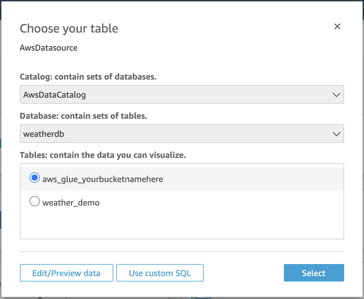

Click Edit/Preview data to preview the dataset contents. You could easily exclude some columns from the dataset or perhaps filter some non-production data away from the analyses. You could even join several datasets from different sources.

We will not do any of that now, but from the top-left corner of the window, select Query mode: SPICE. It means that QuickSight will load all data from our S3 bucket in memory for super-fast data visualization. Every QuickSight account includes 1GB of SPICE memory, and you can purchase more if needed. 1GB is plenty for our small weather dataset.

Click Save & visualize button, and we will start to see miracles!

9. Visualize your weather data

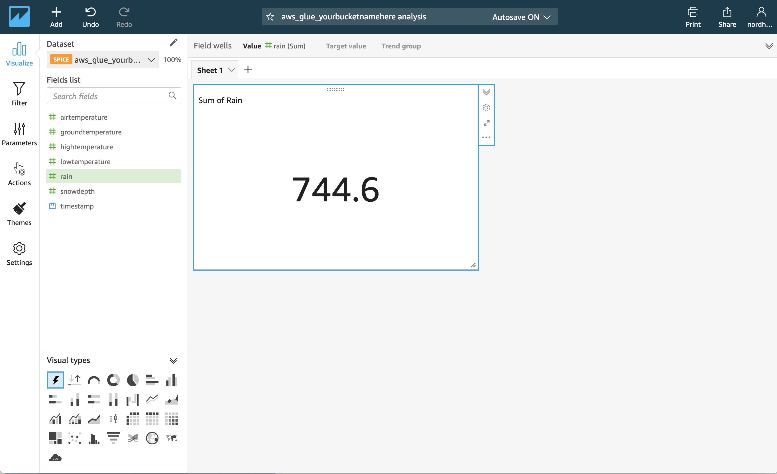
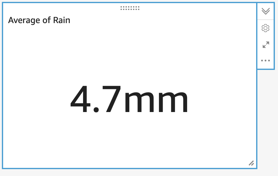
A new Analysis will open up with one sheet and one empty Visual in it. You can see all data fields on the left-hand side. Drag and drop the #rain field to the visual. The visual automatically detects that the field is numeric and calculates the sum of all rain data that we have.

Click the Field wells on top of the Analysis and change the Value from rain (Sum) to rain (Average):

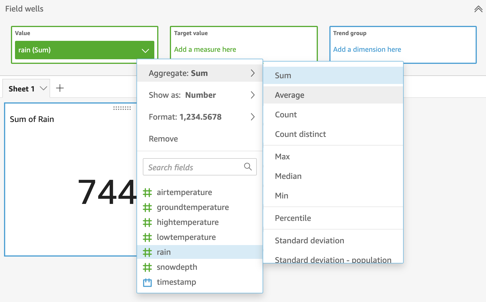
From the same menu, change the number format so that it has one decimal place and mm as units.

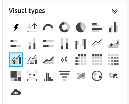
Let’s add one more graph to the page. Click Add from the top navigation and select Add visual. We want to make a traditional weather diagram that combines rain amount bars with a temperature graph. So activate the new visual by clicking it, and then click Clustered bar combo chart from Visual types menu.

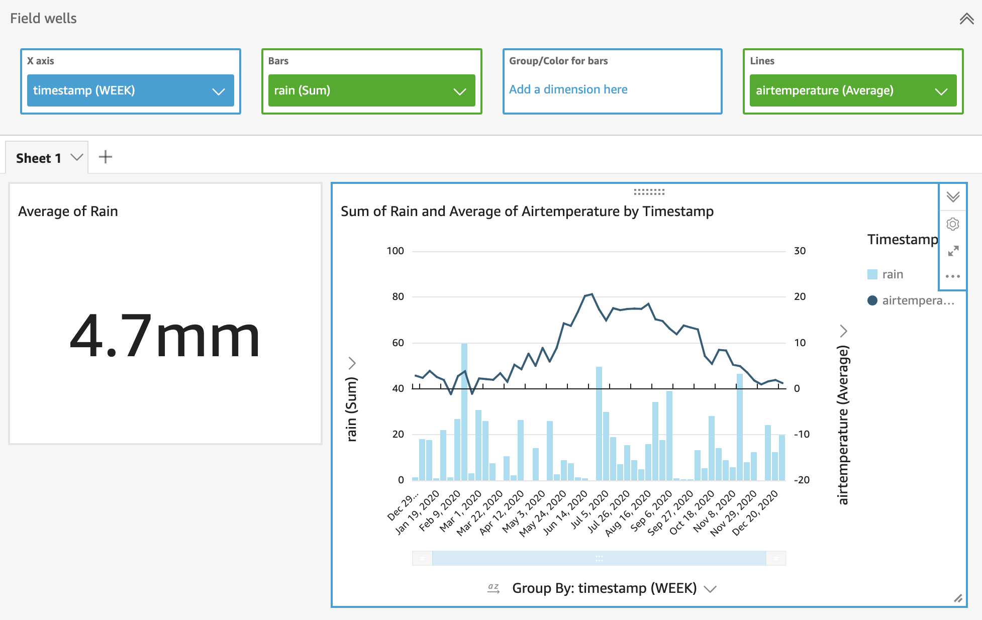
Open Field wells from to of the analysis, and drag and drop needed data to correct fields, and set the correct aggregation for each data:

Field Data field Aggregation

---

X axis timestamp Week
Bars rain Sum
Lines airtemperature Average

There! It seems that it wasn’t that cold in Helsinki in 2020, and the best moment to be on summer holiday would be at the end of June if you prefer warm weather but less water :-)

Closing notes

That was a fun journey. Quite a few steps, but none of those were tough ones. As you can witness, coding was not needed at all! In real life, as more data is saved to DynamoDB, you would need to set a schedule for the Glue job to transfer new and changed data to S3, for example, once per day.

And we have only just touched the surface of capabilities that AWS Glue has to offer on data transformation. And the same applies to QuickSight capabilities. So more NordHero articles are coming up deep-diving in data transformation and BI.

Final note: Please remember to remove all data and services we have put up for this demo if you don’t need the resources anymore. Especially remember to close the QuickSight account within the free trial period if you don’t wish to continue using the service for your business. You can close your QuickSight account by clicking your avatar in the top right corner of QuickSight UI and selecting Manage QuickSight/Account settings/Unsubscribe.